occARU fits Bayesian multispecies occupancy models with count observation models to autonomous recording unit (ARU) data like those derived from camera traps and passive acoustic monitoring. The approach differs from standard occupancy models in that the focus is on quantifying detection rates, rather than treating detection as a nuisance parameter to correct for. The occARU model implements hierarchical species-level random effects with spatial and temporal Gaussian processes, variance decomposition via global-local shrinkage priors, automatically implements single season or dynamic models structures, and is built on Stan via cmdstanr.
Why occARU?
To fit traditional occupancy models with binary observation models, data derived from ARUs is usually collapsed to detection/non-detection events. Models that do use the counts, like N-mixture models for estimating abundance, rely on assumptions that are usually violated with ARU data. occARU models the counts without imposing strict assumptions, while still accounting for species absences at the site level through occupancy modeling.
Installation
Install occARU from GitHub:
# install.packages("remotes")
remotes::install_github("mhollanders/occARU")
occARU requires CmdStan >= 2.36.0. If you have not used Stan before, run:
This checks your C++ toolchain and installs CmdStan automatically.
Getting started
1. Prepare data
make_data() accepts deployment and observation data frames following the camtrapDP format:
data <- make_data(
  deployments = deployments,
  observations = observations,
  failures = failures  # also accepts failure dates per site
  survey_length = 14, # aggregate to 2-weekly survey periods
  thin_minutes = 30  # thin observations to 30 minutes, retaining highest count
  detection_site_predictors = site_predictors,
  survey_predictors = survey_predictors
)
data
#> ── occARU data ─────────────────────────────────────────────────────
#> Sites (I): 30
#> Surveys (J): 114
#> Deployment span: 2019-11-06 to 2024-03-06
#> Regions (R): 3
#> Species (S): 6
#> Detections: 11463
#> Site coordinates: yes
#> Survey length: 14 days
#> Thinning: 30 minutes
#> Occupancy predictors: 0
#> Detection site predictors: 5
#>   Continuous: 3
#>   Categorical: 1
#>   Ordinal: 1
#> Survey predictors: 4
#>   Continuous: 3
#>   Categorical: 0
#>   Ordinal: 1
2. Fit a model
# set some priors for hyperparameters (unspecified use defaults)
priors <- set_priors(
  psi_bar = c(1, 2),  # Beta(1, 2) for mean occupancy
  mu_W = c(3, 0, 1)   # Student-t+(3, 0, 1) for log detection variance
)
#> ── occARU priors ───────────────────────────────────────────────────────────
#> psi_bar: Beta(1, 2)
#> mu_bar: Gamma(1, 1)
#> q_bar: Gamma(1, 3)
#> psi_W: Student-t+(3, 0, 1)
#> mu_W: Student-t+(3, 0, 1)
#> psi_theta: Gamma(1, 1)
#> ...

# fit the model
fit <- occARU(data, prior = priors)
By default this fits a model with spatial and temporal Gaussian processes, Dirichlet variance decomposition, and Poisson observation model, initialised with Pathfinder across 4 chains. See ?occARU and ?set_priors to customise the model structure and priors.
3. Check some output
# site occupancy and detection rates
plot_sites(fit)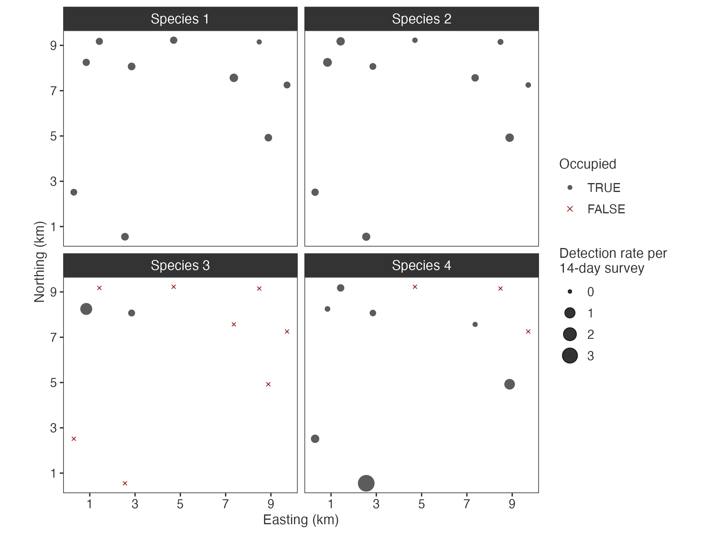
# temporal detection trends
plot_surveys(fit, species = c("Species 1", "Species 2"))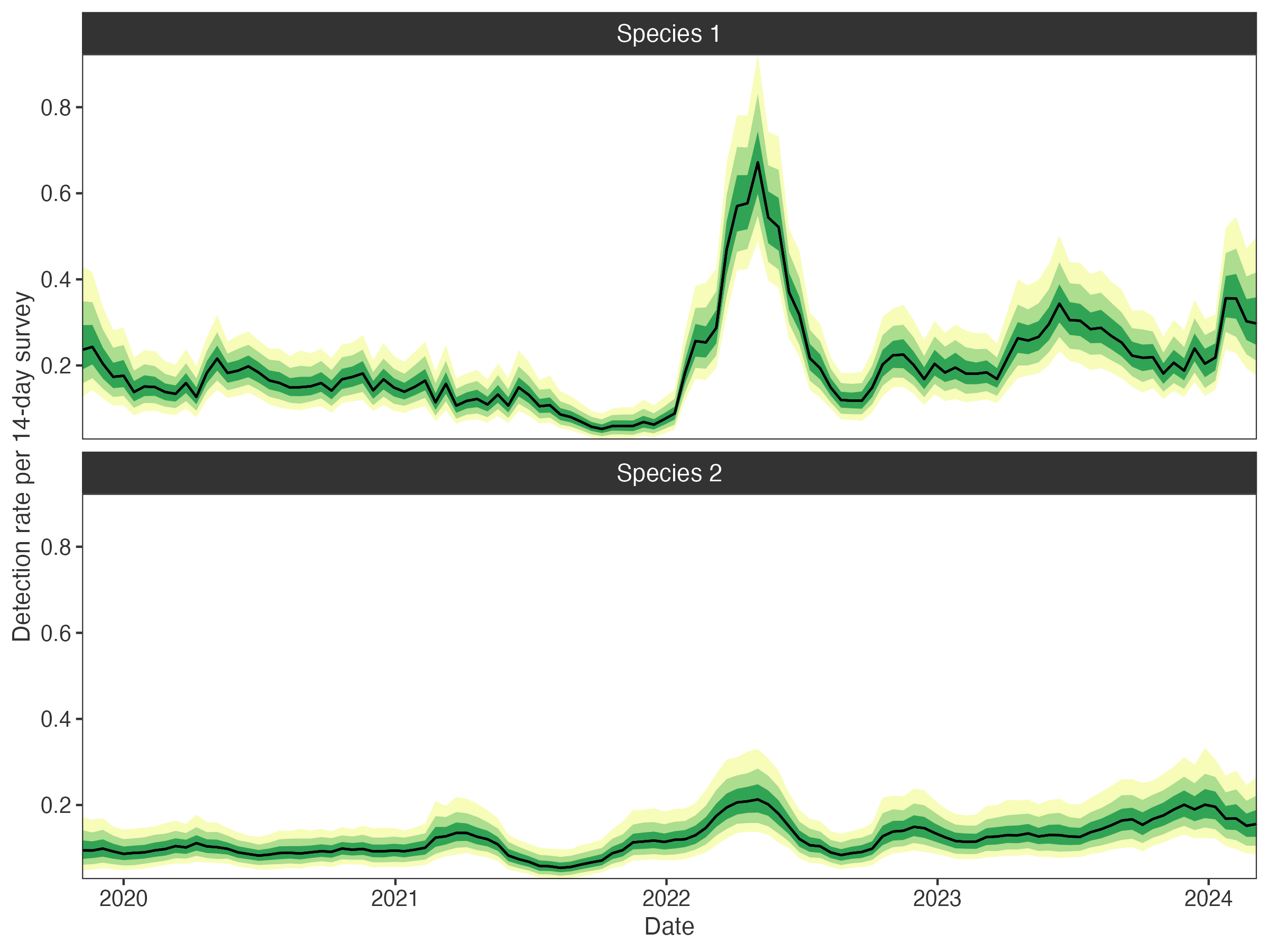
Key design choices in occARU are multispecies random site and survey effects implemented as hierarchical multivariate Gaussian processes. Interspecific correlations are estimated for responses to predictors and random effects to explore species interactions.
# variance partitions
plot_partitions(fit, scales = TRUE)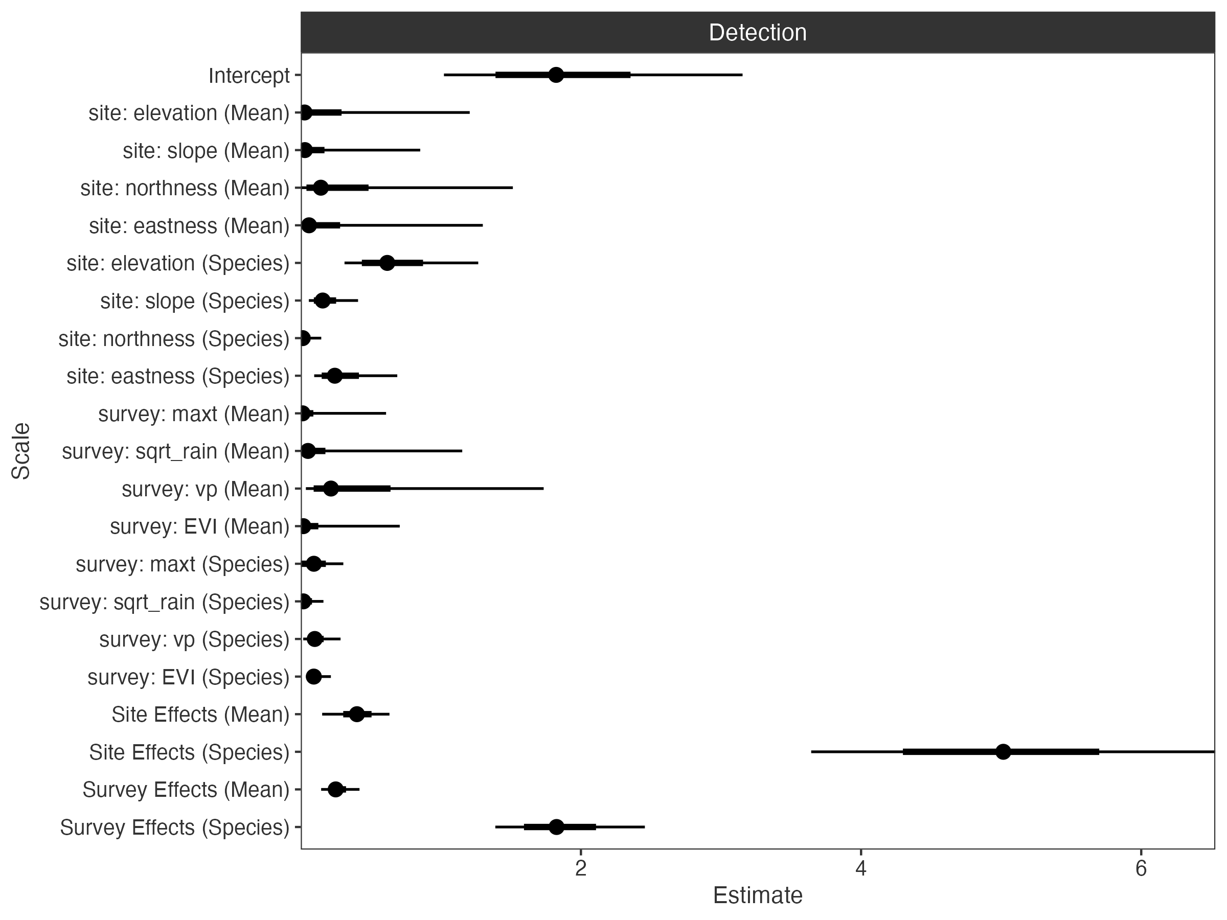
Global-local shrinkage priors are used to handle model complexity through variance decomposition of the occupancy and detection linear predictors.
4. Interrogate
# use PSIS-LOO-CV on the site-by-species level log likelihood
fit$loo("log_lik2")  # log_lik2 uses Monte Carlo integration of random effects

# posterior predictive checking with rootograms of site-by-species counts
pp_check(fit, level = "Q")

# check prior sensitivity using power-scaling
priorsense::powerscale_plot_dens(fit$draws("log_lik", "lprior", "psi_bar"))
The model stores marginal site-by-species log likelihoods (log_lik), the log prior density (lprior), and posterior predictions for the full detection history (yrep) or aggregated site-by-species counts (Qrep). Optionally, Monte Carlo integration over site and observation-level random effects produces marginal log likelihoods (log_lik2) with improved PSIS-LOO-CV performance.